

SITCOMTN-156
ComCam: The impact of using a different number of donut pairs and binning settings on the wavefront retrieval#
In this document we investigate the effect of choosing a different number of donut pairs per LsstComCam detector for wavefront sensing using Danish or TIE algorithms. We also test the impact of binning the image data.
Last verified to run: 03/10/2025
Versions:
lsst_distrib w_2025_08 (ext, cvmfs)
ts_wep v13.4.1
Imports#
from astropy.table import Table
from astropy.visualization import ZScaleInterval
from astropy.time import Time
import astropy.units as u
from copy import copy
from lsst.daf.butler import Butler
from lsst.ts.wep.utils import makeDense, makeSparse, convertZernikesToPsfWidth, binArray
import matplotlib.pyplot as plt
import numpy as np
from tqdm import tqdm
import os
Input#
We use the existing donut stamps in /repo/main, collection u/brycek/aosBaseline_step1a. This run ISR and ts_wep donut detection and cutouts on the ComCam data where exposure.observation_type = 'cwfs'. The pipetask used step1a of comCamBaselineUSDF_Danish.yaml , which imports comCamBaselineUSDF_Danish.yaml . The combined pipeline config for step1a included:
instrument: lsst.obs.lsst.LsstComCam
  isr:
    class: lsst.ip.isr.IsrTaskLSST
    config:
      # Although we don't have to apply the amp offset corrections, we do want
      # to compute them for analyzeAmpOffsetMetadata to report on as metrics.
      doAmpOffset: True
      ampOffset.doApplyAmpOffset: False
      # Turn off slow steps in ISR
      doBrighterFatter: False
      # Mask saturated pixels,
      # but turn off quadratic crosstalk because it's currently broken
      doSaturation: True
      crosstalk.doQuadraticCrosstalkCorrection: False
  generateDonutDirectDetectTask:
    class: lsst.ts.wep.task.generateDonutDirectDetectTask.GenerateDonutDirectDetectTask
    config:
      donutSelector.useCustomMagLimit: True
      donutSelector.sourceLimit: -1
  cutOutDonutsScienceSensorGroupTask:
    class: lsst.ts.wep.task.cutOutDonutsScienceSensorTask.CutOutDonutsScienceSensorTask
    config:
      python: |
        from lsst.ts.wep.task.pairTask import GroupPairer
        config.pairer.retarget(GroupPairer)
      donutStampSize: 200
      initialCutoutPadding: 40
This resulted in 22452 unique dataset references with donutStampsExtra, donutStampsIntra (i.e. combinations of exposure - detector data elements that cab be accessed by butler).
Data Processing#
The above was processed using batch processing service (bps) at the US Data Facility (USDF). Following the ssh to s3df and one of the submission nodes (eg. sdfiana012), we setup the LSST Science Pipelines and the AOS packages. Ensuring the presence of site_bps.yaml in the submission directory containing
site:
  s3df:
    profile:
      condor:
        +Walltime: 7200
we obtain glidee in nodes with
allocateNodes.py -v -n 15 -c 64 -m 60:00:00 -q milano -g 1800 s3df --account rubin:commissioning
The basis of employed pipetask configs are comCamBaselineUSDF_Danish.yaml and comCamBaselineUSDF_TIE.yaml.
These were used to create lsstComCamPipelineDanish.yaml containing:
description: rerun lsstComCam Danish baseline with different binning
instrument: lsst.obs.lsst.LsstComCam
tasks:
  calcZernikesTask:
    class: lsst.ts.wep.task.calcZernikesTask.CalcZernikesTask
    config:
      python: |
        from lsst.ts.wep.task import EstimateZernikesDanishTask
        config.estimateZernikes.retarget(EstimateZernikesDanishTask)
      donutStampSelector.maxFracBadPixels: 2.0e-4
      estimateZernikes.binning: 1
      estimateZernikes.nollIndices:
        [4, 5, 6, 7, 8, 9, 10, 11, 12, 13, 14, 15, 20, 21, 22, 27, 28]
      estimateZernikes.saveHistory: False
      estimateZernikes.lstsqKwargs:
        ftol: 1.0e-3
        xtol: 1.0e-3
        gtol: 1.0e-3
      donutStampSelector.maxSelect: -1
  aggregateZernikeTablesTask:
    class: lsst.donut.viz.AggregateZernikeTablesTask
  aggregateDonutTablesGroupTask:
      class: lsst.donut.viz.AggregateDonutTablesTask
      config:
          python: |
              from lsst.ts.wep.task.pairTask import GroupPairer
              config.pairer.retarget(GroupPairer)
  aggregateAOSVisitTableTask:
    class: lsst.donut.viz.AggregateAOSVisitTableTask

  plotAOSTask:
    class: lsst.donut.viz.PlotAOSTask
    config:
      doRubinTVUpload: false

  aggregateDonutStampsTask:
    class: lsst.donut.viz.AggregateDonutStampsTask

  plotDonutTask:
   class: lsst.donut.viz.PlotDonutTask
   config:
     doRubinTVUpload: false
and lsstComCamPipelineTie.yaml containing:
description: rerun lsstComCam TIE baseline with different binning
instrument: lsst.obs.lsst.LsstComCam
tasks:
  calcZernikesTask:
    class: lsst.ts.wep.task.calcZernikesTask.CalcZernikesTask
    config:
      estimateZernikes.binning: 1
      estimateZernikes.nollIndices: [4, 5, 6, 7, 8, 9, 10, 11, 12, 13, 14, 15, 20, 21, 22, 27, 28]
      estimateZernikes.convergeTol: 10.0e-9
      estimateZernikes.compGain: 0.75
      estimateZernikes.compSequence: [4, 4, 6, 6, 13, 13, 13, 13]
      estimateZernikes.maxIter: 50
      estimateZernikes.requireConverge: True
      estimateZernikes.saveHistory: False
      estimateZernikes.maskKwargs: { "doMaskBlends": False }
      donutStampSelector.maxFracBadPixels: 2.0e-4
      donutStampSelector.maxSelect: -1

  aggregateZernikeTablesTask:
    class: lsst.donut.viz.AggregateZernikeTablesTask
  aggregateDonutTablesGroupTask:
      class: lsst.donut.viz.AggregateDonutTablesTask
      config:
          python: |
              from lsst.ts.wep.task.pairTask import GroupPairer
              config.pairer.retarget(GroupPairer)
  aggregateAOSVisitTableTask:
    class: lsst.donut.viz.AggregateAOSVisitTableTask

  plotAOSTask:
    class: lsst.donut.viz.PlotAOSTask
    config:
      doRubinTVUpload: false

  aggregateDonutStampsTask:
    class: lsst.donut.viz.AggregateDonutStampsTask

  plotDonutTask:
   class: lsst.donut.viz.PlotDonutTask
   config:
     doRubinTVUpload: false
Main modification to the original ts_wep pipeline was to set estimateZernikes.nollIndices to be identical for Danish and TIE versions.
Image binning takes place at the image level, and is possible for both Danish and TIE algorithms. We change the image binning by seting estimateZernikes.binning to 1 to 2 or 4, creating _binning_1, etc versions of each pipeline.
We submit all with bps for Danish:
bps submit site_bps.yaml -b /repo/main -i u/brycek/aosBaseline_step1a,LSSTComCam/calib/unbounded -o u/scichris/aosBaseline_danish_binning_1 -p /sdf/data/rubin/shared/scichris/DM-48441_N_donuts_LsstComCam/lsstComCamPipelineDanish_binning_1.yaml

bps submit site_bps.yaml -b /repo/main -i u/brycek/aosBaseline_step1a,LSSTComCam/calib/unbounded -o u/scichris/aosBaseline_danish_binning_2 -p /sdf/data/rubin/shared/scichris/DM-48441_N_donuts_LsstComCam/lsstComCamPipelineDanish_binning_2.yaml

bps submit site_bps.yaml -b /repo/main -i u/brycek/aosBaseline_step1a,LSSTComCam/calib/unbounded -o u/scichris/aosBaseline_danish_binning_2 -p /sdf/data/rubin/shared/scichris/DM-48441_N_donuts_LsstComCam/lsstComCamPipelineDanish_binning_4.yaml
and TIE:
bps submit site_bps.yaml -b /repo/main -i u/brycek/aosBaseline_step1a,LSSTComCam/calib/unbounded -o u/scichris/aosBaseline_tie_binning_1 -p /sdf/data/rubin/shared/scichris/DM-48441_N_donuts_LsstComCam/lsstComCamPipelineTie_binning_1.yaml

bps submit site_bps.yaml -b /repo/main -i u/brycek/aosBaseline_step1a,LSSTComCam/calib/unbounded -o u/scichris/aosBaseline_tie_binning_2 -p /sdf/data/rubin/shared/scichris/DM-48441_N_donuts_LsstComCam/lsstComCamPipelineTie_binning_2.yaml

bps submit site_bps.yaml -b /repo/main -i u/brycek/aosBaseline_step1a,LSSTComCam/calib/unbounded -o u/scichris/aosBaseline_tie_binning_4 -p /sdf/data/rubin/shared/scichris/DM-48441_N_donuts_LsstComCam/lsstComCamPipelineTie_binning_4.yaml
Binning and image resolution#
Configuring estimateZernikes.binning to a value larger than 1 means that both intra- and extra-focal images are reduced in resolution before being analyzed by the chosen algorithm (Danish or TIE). An example simulated image of ComCam binned by a factor of x1 (no binning), x2, x4, is shown below:
butlerRootPath = "/sdf/data/rubin/repo/aos_imsim/"
butler = Butler(butlerRootPath)
registry = butler.registry
refs = butler.query_datasets(
    "donutStampsExtra",
    collections=["WET-001_lsstComCam_TIE_6001_6200_bps"],
    where="instrument='LSSTComCam' and detector = 4",
)
donutStampsExtra = butler.get(
    "donutStampsExtra",
    dataId=refs[60].dataId,
    collections=["WET-001_lsstComCam_TIE_6001_6200_bps"],
)
fig, ax = plt.subplots(1, 3, figsize=(10, 4))
image = donutStampsExtra[0].stamp_im.image.array

for i, binning in enumerate([1, 2, 4]):
    binned_image = binArray(image, binning)
    ax[i].imshow(binned_image, origin="lower")
    ax[i].set_title(f"binning: {binning}")
ax[0].set_ylabel("y [px]")
fig.suptitle("Simulated ComCam extra-focal donut, R22_S11")
fig.text(
    0.5,
    0.1,
    "x [px]",
)
Text(0.5, 0.1, 'x [px]')
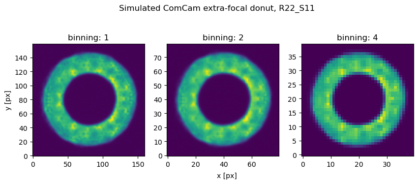
The reduction of resolution degrades the content of information, and potentially decreases the task execution time, as shown below.
Impact on runtime#
To compare runtime of different estimateZernikes.binning settings, we read the information stored in task_metadata, and task_log dataset types. Due to the number of involved visits, we ran the attached scripts read_runtime and clean_runtime via slurm individually per method / binning.
results_timing = {}
for method in ['tie', 'danish']:
    results_timing[method] = {}
    for binning in [1, 2, 4]:

        fname = f"DM-49211_u_scichris_aosBaseline_binning_{binning}_{method}_timing_table.txt"
        if os.path.exists(fname):
            results_timing[method][binning] = Table.read(fname, format='ascii')
        else:
            print(f"Need to first execute python read_runtime and clean_runtime in the technote github repository")
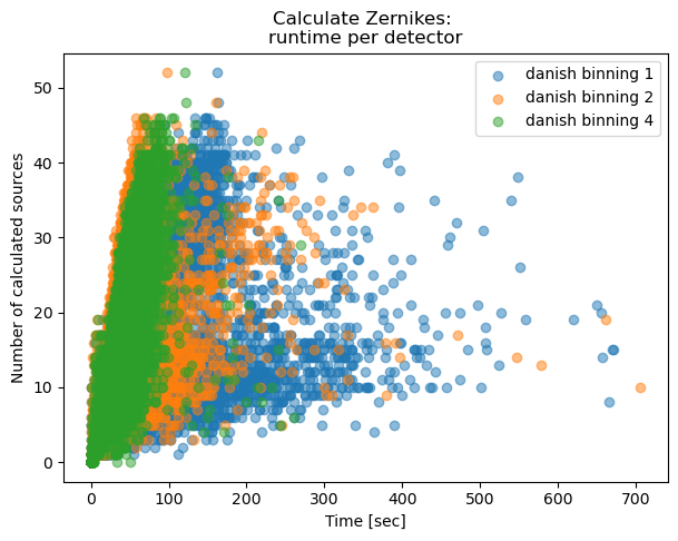
The execution time is obtained from calcZernikesTask_metadata, between quantum/prepUtc and quantum/endUtc
fig,ax = plt.subplots(1,1,figsize=(7,5))
method = 'danish'
for binning in  [1,2,4]:
    results =  results_timing[method]
    ax.scatter(results_timing[method][binning]['cwfsTime'], results_timing[method][binning]['NobjCalc'], label=f'{method} binning {binning}',
              alpha=0.5)
ax.legend()
ax.set_xlabel('Time [sec]')
ax.set_ylabel('Number of calculated sources')
ax.set_title('Calculate Zernikes: \nruntime per detector')
Text(0.5, 1.0, 'Calculate Zernikes: \nruntime per detector')
fig,ax = plt.subplots(1,1,figsize=(7,5))
method = 'tie'
for binning in  [1,2,4]:
    results =  results_timing[method]
    ax.scatter(results_timing[method][binning]['cwfsTime'], results_timing[method][binning]['NobjCalc'], label=f'{method} binning {binning}',
              alpha=0.5)
ax.legend()
ax.set_xlabel('Time [sec]')
ax.set_ylabel('Number of calculated sources')
ax.set_title('Calculate Zernikes: \nruntime per detector')
Text(0.5, 1.0, 'Calculate Zernikes: \nruntime per detector')
We can divide the execution time per number of sources, and plot a histogram per method / binning:
for method in results_timing.keys():
    fig,ax = plt.subplots(1,1,figsize=(7,5))
    for binning in  [1,2,4]:
        ls = 'dashed' if method == 'tie' else 'solid'
        cwfs_time = np.array(results_timing[method][binning]['cwfsTime'])
        nobj_calc = np.array(results_timing[method][binning]['NobjCalc'])
        m = nobj_calc>0
        time_per_obj = cwfs_time[m] / nobj_calc[m]
        ax.hist(time_per_obj, histtype='step', lw=3, ls=ls, label=f'{method} binning {binning}', alpha=0.8,
               bins=35, range=(0,20)
               )

        print(f'{method}, binning x{binning}, median execution time: {np.median(time_per_obj)}')
    ax.set_xlabel('Time per source) [sec]')
    ax.set_ylabel('Count')
    ax.legend()
tie, binning x1, median execution time: 2.096354374999887
tie, binning x2, median execution time: 0.6352792857156889
tie, binning x4, median execution time: 0.44021016666695445
danish, binning x1, median execution time: 3.813606406593311
danish, binning x2, median execution time: 1.8558818888883977
danish, binning x4, median execution time: 2.37407587857106
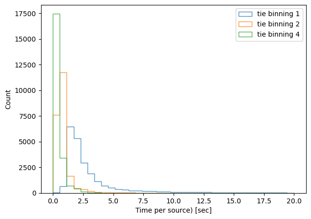
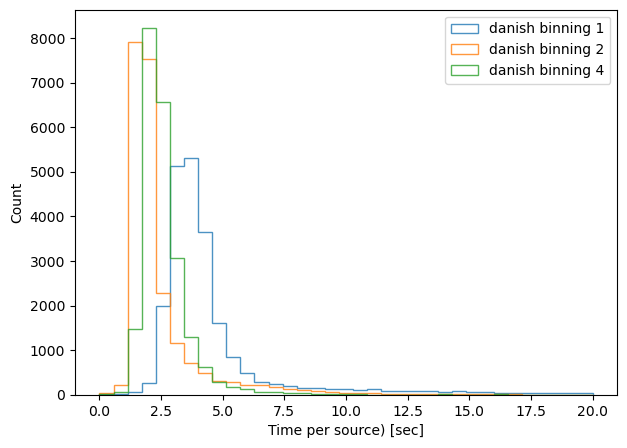
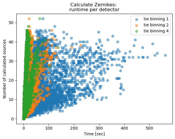
As expected, binning reduces the task execution time. Both methods are shown in the same scale, highlighting the fact that the TIE algoritm is slightly faster than Danish (with x2 binning, median 0.63 sec/source for TIE vs 1.85 sec/source for Danish). Next we consider an extent to which this image quality degradation affects the inferred wavefront, selecting only datasets with multiple donut stamps selected per detector.
Sample Selection#
The initial dataset includes all data labelled as defocal:
butler = Butler("/repo/main")
input_collection =  "u/brycek/aosBaseline_step1a" # only data labelled with observation_type as cwfs
refs = butler.query_datasets('donutStampsExtra',  collections=[input_collection], limit=None)
len(refs)
22452
It corresponds to 2500 unique visits:
visits, count =  np.unique(list(ref.dataId["visit"] for ref in refs), return_counts=True)
print(len(np.unique(visits)))
2500
However, only 2474 have data for all 9 detectors at the same time:
good_visits = visits[np.where(count == 9)]
print(len(np.unique(good_visits)))
2474
Each bps run above produced donutQualityTable with data for both intra and extra-focal exposure in the same group, such as:
wep_collection = 'u/scichris/aosBaseline_danish_binning_1'
refs = butler.query_datasets('zernikes',  collections=[wep_collection], limit=1)
donutQualityTable = butler.get('donutQualityTable', dataId=refs[0].dataId, collections=[wep_collection])
donutQualityTable[:5]
| SN | ENTROPY | FRAC_BAD_PIX | SN_SELECT | ENTROPY_SELECT | FRAC_BAD_PIX_SELECT | FINAL_SELECT | DEFOCAL_TYPE |
|---|---|---|---|---|---|---|---|
| float64 | float64 | float64 | bool | bool | bool | bool | str5 |
| 5137.41357421875 | 1.31518296329074 | 0.0 | True | True | True | True | extra |
| 1318.29467773438 | 3.24980303079286 | 0.0 | True | True | True | True | extra |
| 978.061645507812 | 3.5127111308061 | 0.0 | False | True | True | False | extra |
| 924.204772949219 | 3.52984575330561 | 0.0 | False | True | True | False | extra |
| 791.558532714844 | 3.75901379543286 | 0.0 | False | True | True | False | extra |
Each donutQualityTable is created by the donutStampSelector, called by calcZernikesTask during wavefront estimation. It combines individual donut stamp information calculated by cutOutDonutsBase during the cutout stage, and applies selection criteria (such as maxFracBadPixels or maxEntropy) to set FINAL_SELECT flag that passes only select donut stamp pairs to estimateZernikes task. Using the FINAL_SELECT column, we count the number of donuts per detector that were admitted in the Zernike estimation:
# Get information about how many donuts made it through selection criteria
# by reading all `donutQualityTables` :
butler = Butler('/repo/main')
wep_collection = 'u/scichris/aosBaseline_danish_binning_1'

# First , want to make sure that all detectors got processed per visit.
refs = butler.query_datasets('zernikes',  collections=[wep_collection], limit=None)
visits, count =  np.unique(list(ref.dataId["visit"] for ref in refs), return_counts=True)
good_visits = visits[np.where(count == 9)]
print(f'{len(good_visits)} / {len(visits)} have data for all detectors')

nDonutsQualityTable = []
nDonutsQualityTableIntra = []
nDonutsQualityTableExtra = []
visits = []
dets = []

for ref in tqdm(refs, desc="Processing"):
    if ref.dataId["visit"] in good_visits:
        # Note: there's one `donutQualityTable` for intra and extra-focal pair.
        donutQualityTable = butler.get('donutQualityTable', dataId=ref.dataId, collections=[wep_collection])
        nDonutsQualityTable.append(np.sum(donutQualityTable['FINAL_SELECT']))
        donutQualityTableExtra = donutQualityTable[donutQualityTable['DEFOCAL_TYPE'] == 'extra']
        donutQualityTableIntra = donutQualityTable[donutQualityTable['DEFOCAL_TYPE'] == 'intra']
        nDonutsQualityTableIntra.append(np.sum(donutQualityTableIntra['FINAL_SELECT']))
        nDonutsQualityTableExtra.append(np.sum(donutQualityTableExtra['FINAL_SELECT']))
        visits.append(ref.dataId['visit'])
        dets.append(ref.dataId['detector'])

#Store the full table:
donutQualityTableNdonuts = Table(data=[nDonutsQualityTable, nDonutsQualityTableIntra,
                                       nDonutsQualityTableExtra,
                                       visits,dets],
                                 names=['Ndonuts', 'NdonutsIntra', 'NdonutsExtra',
                                                            'visit', 'detector'])
fnameDonutTable = 'u_scichris_aosBaseline_danish1_donutQualityTable_N_donuts.txt'
donutQualityTableNdonuts.write(fnameDonutTable, format='ascii')
Of 2474 visits, 2457 have processed Zernike data for all 9 detectors. We select a subset that has at least 9 donuts in each detector:
fnameDonutTable = 'u_scichris_aosBaseline_danish1_donutQualityTable_N_donuts.txt'
donutQualityTableNdonuts = Table.read(fnameDonutTable, format='ascii')

m = (donutQualityTableNdonuts['NdonutsIntra'] > 8 ) * ( donutQualityTableNdonuts['NdonutsExtra'] > 8 )
donutTableSubset = donutQualityTableNdonuts[m]

good_visits  = []
for visit in np.unique(donutTableSubset['visit']):
    rows  = donutTableSubset[donutTableSubset['visit'] == visit]
    if len(rows) == 9: # all detectors fulfill the number of donuts criterion
        good_visits.append(visit)
mask = np.isin(donutTableSubset['visit'] , good_visits)
donutQualityTableSel = donutTableSubset[mask]
fnameDonutTableSel = 'u_scichris_aosBaseline_danish1_donutQualityTable_N_donuts_select.txt'
donutQualityTableSel.write(fnameDonutTableSel, format='ascii')
print(f'The table includes {len(donutQualityTableSel)} dataRefs, with {len(good_visits)} unique visits')
The table includes 5166 dataRefs, with 574 unique visits
Data analysis#
We reorganize all zernikes tables for selected visits using the read_zernikes_comcam script, and subsequently add donut magnitude converting source_flux that is stored in each donutQualityTable:
path_cwd = os.getcwd()
fname = os.path.join(path_cwd, f'u_scichris_aosBaseline_tie_danish_zernikes_tables_604.npy')
results_visit = np.load(fname, allow_pickle=True).item()

fnameSelectionTable = 'u_scichris_aosBaseline_danish1_donutQualityTable_N_donuts_select.txt'
donutQualityTableSel = Table.read(fnameSelectionTable, format='ascii')

visits_calculated = np.unique(list(results_visit.keys()))
visits_selected  = np.unique(donutQualityTableSel['visit'])
visits_available = visits_selected[np.isin(visits_selected, visits_calculated)]
# Setup butler
butler =  Butler('/repo/main')

results_visit_mags = {}
for visit  in tqdm(visits_available, desc="Processing"):

    results_mags = {}
    for detector in range(9):

        dataId = {'instrument':'LSSTComCam', 'detector':detector,
                'visit':visit
             }
        donutTableExtra = butler.get('donutTable', dataId=dataId, collections=['u/brycek/aosBaseline_step1a'])
        donutQualityTable = butler.get('donutQualityTable', dataId=dataId, collections=['u/scichris/aosBaseline_tie_binning_1'])

        extraDonuts = donutQualityTable[donutQualityTable['DEFOCAL_TYPE'] == 'extra']
        extraDonuts['index'] = np.arange(len(extraDonuts))

        extraIndices = extraDonuts[extraDonuts['FINAL_SELECT']]['index']
        idxExtra = np.array(extraIndices.data, dtype=int)

        donutTableExtraSelect = donutTableExtra[idxExtra]
        mags  = (donutTableExtra[idxExtra]['source_flux'].value * u.nJy).to_value(u.ABmag)

        results_mags[detector] = { 'donutStampsExtraMag':mags}
    results_visit_mags[visit] = results_mags

Nvisits = len(visits_available)
file = f'u_scichris_aosBaseline_tie_danish_mag_visit_{Nvisits}.npy'
np.save(file, results_visit_mags, allow_pickle=True)
Increasing the number of donuts#
We plot the average of N donuts pairs, as we start from N=1 (single donut pair), to N=9 (average of nine donut pairs). Each panel corresponds to an individual LsstComCam detector:
visit = visits_available[3]

Nmin = 1

fig,axs = plt.subplots(3,3,figsize=(16,10))
ax = np.ravel(axs)
method = 'danish1'
for Nmax in range(1,10):
    results = results_visit[visit][method]

    # iterate over detectors
    for i in range(9):
        zernikes_all = results[i]

        # select only those donut pairs that were actually used
        zernikes = zernikes_all[zernikes_all['used'] == True]

        if Nmax+1 <= len(zernikes):
            # Select row or a range of rows
            rows = zernikes[Nmin:Nmax]

            # read off which modes were fitted
            zk_cols = [col for col in zernikes.columns if col.startswith('Z')]
            zk_modes = [int(col[1:]) for col in zk_cols]
            zk_fit_nm_median = [np.median(rows[col].value) for col in zk_cols]

            ax[i].plot(zk_modes, zk_fit_nm_median, marker='d', label=f'<{Nmax} pairs> ')

            ax[i].set_xticks(np.arange(4,29,step=2))
            ax[i].axhline(0,ls='--', c='red')

        else:
            raise ValueError(f'Nmax= {Nmax} > {len(zernikes)} ')

# Also plot the stored average value which is the 0th row
for i in range(9):
    # select zernikes for that detector
     zernikes = results_visit[visit][method][i]
     ax[i].set_title(i)
    # select the average
     rows = zernikes[0]
     zk_fit_nm_median = [np.median(rows[col].value) for col in zk_cols]
     ax[i].plot(zk_modes, zk_fit_nm_median, marker='d', lw=3, c='red', label='stored average',
               alpha=0.7)
ax[2].legend(bbox_to_anchor = [1.5,0.5])


fig.text(0.5,0.05, 'Zk mode')
fig.text(0.05,0.5,' Zk value [nm]', rotation='vertical')
fig.subplots_adjust(hspace=0.3)
fig.suptitle(f'DM-48441:  comCam, visit {visit}, N donuts, {method} ')
Text(0.5, 0.98, 'DM-48441: comCam, visit 2024102700040, N donuts, danish1 ')
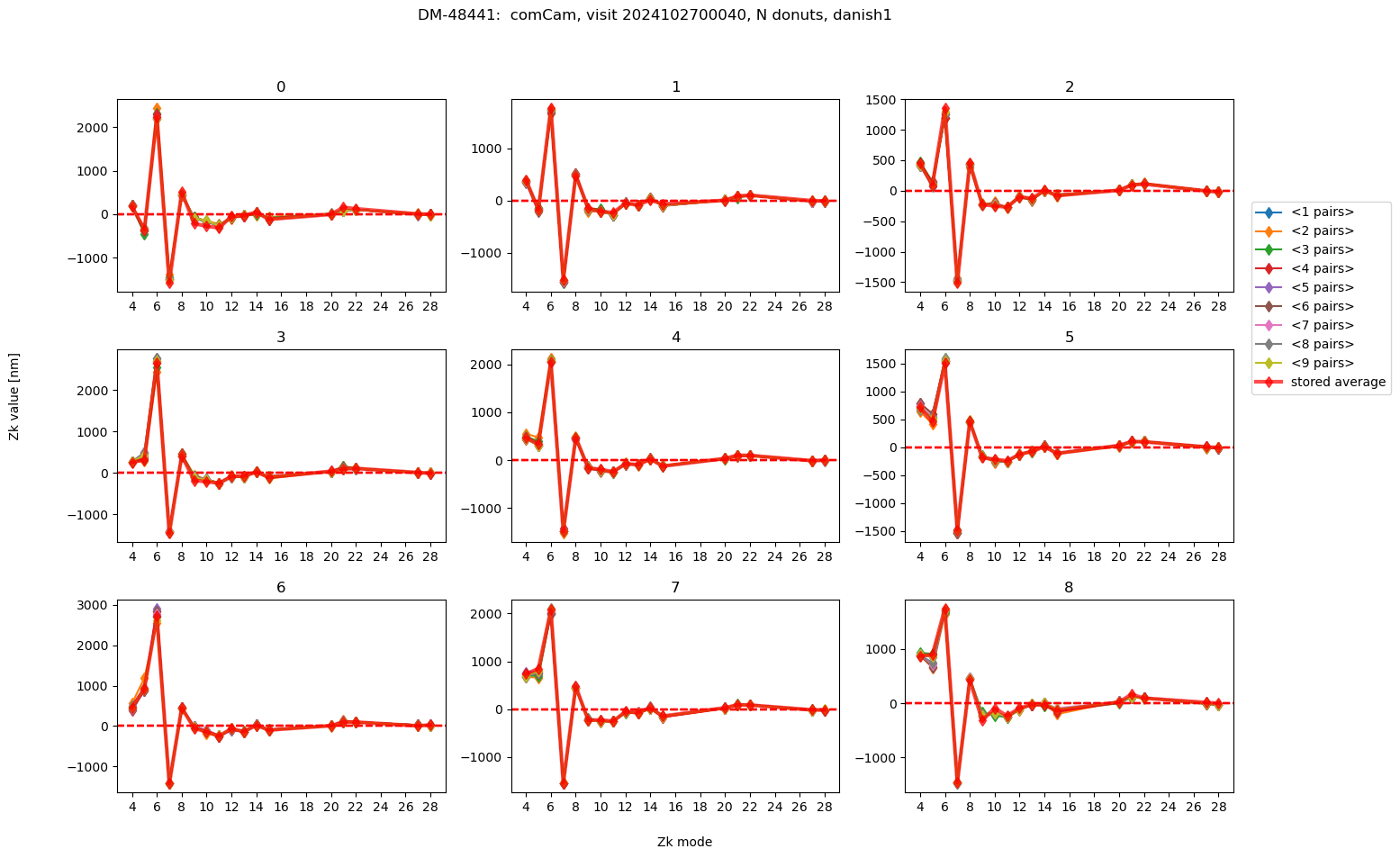
As we see, on an absolute scale the deviations are very small. Illustrate their range by plotting the deviation from the average using all 9 donuts:
Nmin = 1

fig,axs = plt.subplots(3,3,figsize=(16,10))
ax = np.ravel(axs)

for Nmax in range(1,10):
    # plot for  each detector just the first donut pair
    for i in range(9):
        # read off which modes were fitted
        zernikes_all = results_visit[visit][method][i]

        # select only those zernikes that were actually used
        zernikes = zernikes_all[zernikes_all['used'] == True]
        zk_cols = [col for col in zernikes.columns if col.startswith('Z')]
        zk_modes = [int(col[1:]) for col in zk_cols]

        # Calculate the final average of N donut pairs
        rows = zernikes[Nmin:10]
        zk_fit_nm_avg  = [np.median(rows[col].value) for col in zk_cols]

        if Nmax+1 <= len(zernikes):
            # Select row or a range of rows
            rows = zernikes[Nmin:Nmax+1]

            # read off which modes were fitted
            zk_cols = [col for col in zernikes.columns if col.startswith('Z')]
            zk_modes = [int(col[1:]) for col in zk_cols]
            zk_fit_nm_median = [np.median(rows[col].value) for col in zk_cols]

            ax[i].plot(zk_modes, np.array(zk_fit_nm_median) - np.array(zk_fit_nm_avg), marker='d', label=f'<{Nmax} pairs>-avg ')
            ax[i].set_title(i)
            ax[i].set_xticks(np.arange(4,29,step=2))
            ax[i].axhline(0,ls='--', c='red')

        else:
            raise ValueError(f'Nmax= {Nmax} > {len(zernikes)} ')

ax[2].legend(bbox_to_anchor=[1.5,0.6], title='<N donuts> - average')
fig.text(0.5,0.05, 'Zk mode')
fig.text(0.05,0.5,  r'$\Delta$'+'Zk value [nm]', rotation='vertical')
fig.subplots_adjust(hspace=0.3)
fig.suptitle(f'DM-48441:  comCam, visit {visit}, N donuts, {method} ')
Text(0.5, 0.98, 'DM-48441: comCam, visit 2024102700040, N donuts, danish1 ')
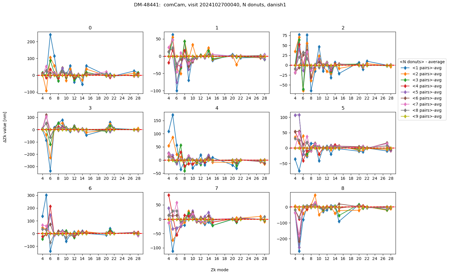
We can summarize that by plotting for each visit the RMS difference between average using N-donut pairs (with N:1,2,3,4, etc) and N=9 (final average). This corresponds to the speed of convergence to the final result:
Nmin = 1  # row 0 is the average
NmaxValue = 10
method = 'tie1'

fig,ax = plt.subplots(1,1,figsize=(7,5))

per_det = []
# iterate over detectors
for i in range(9):
    zernikes = results_visit[visit][method][i]

    # read the available names of Zk mode columns
    zk_cols = [col for col in zernikes.columns if col.startswith('Z')]
    zk_modes = [int(col[1:]) for col in zk_cols]

    # Calculate the final average of N donut pairs
    rows = zernikes[Nmin:NmaxValue]
    zk_fit_nm_avg  = [np.median(rows[col].value) for col in zk_cols]
    rms_diffs_per_det = []

    # iterate over how many donut pairs to include in the average
    for Nmax in range(1,NmaxValue):

        if Nmax+1 <= len(zernikes):
            # Select row or a range of rows
            rows = zernikes[Nmin:Nmin+Nmax]

            # read off which modes were fitted
            zk_fit_nm_median = [np.median(rows[col].value) for col in zk_cols]

            rms_diff =  np.sqrt(
                    np.mean(
                            np.square(
                                        np.array(zk_fit_nm_avg) - np.array(zk_fit_nm_median)
                                     )
                           )
                   )
            rms_diffs_per_det.append(rms_diff)

        else:
            raise ValueError(f'Nmax= {Nmax} > {len(zernikes)} ')
    per_det.append(rms_diffs_per_det)

    # plot the RMS diff for each detector
    ax.plot(range(Nmin,NmaxValue), rms_diffs_per_det, marker='d', label=f'detector {i}', alpha=0.5)

ax.set_xticks(range(Nmin,NmaxValue))
ax.axhline(0,ls='--', c='red')

# Plot detector average
ax.plot(range(Nmin, NmaxValue), np.mean(per_det, axis=0), marker='d', lw=5, alpha=0.6,  label='average' )


ax.set_xlabel('N donut pairs')
ax.set_ylabel(r'$\Delta$ RMS'+' Zk value (all pairs)-N pairs [nm]', )
ax.set_title(f'DM-48441:  comCam, visit {visit}, N donuts, {method} ')
ax.legend()
<matplotlib.legend.Legend at 0x7f26bb4d49b0>
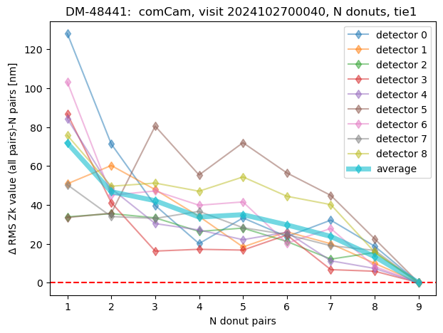
We can calculate this metric for all visits, expressing RMS in both nm and asec:
# calculation of RMS diff
Nmin=1
NmaxValue = 10

rms_visit = {}
rms_visit_asec = {}
count =0
for visit in tqdm(visits_available, desc='Calculating'):
    rms_diffs = {}
    rms_diffs_asec = {}
    for  method  in results_visit[visit].keys():
        results = results_visit[visit][method]
        rms_diffs[method] = {}
        rms_diffs_asec[method] = {}
        for i in range(9):
            zernikes_all = results[i]
            # select only those zernikes that were actually used
            zernikes = zernikes_all[zernikes_all['used'] == True]

            # read the available names of Zk mode columns
            zk_cols = [col for col in zernikes.columns if col.startswith('Z')]

            # read off which modes were fitted
            zk_modes = [int(col[1:]) for col in zk_cols]

            # select not the stored average,
            # but calculate average using all available donuts
            all_rows = zernikes[Nmin:NmaxValue]
            zk_fit_avg_nm  = [np.median(all_rows[col].value) for col in zk_cols]
            zk_fit_avg_nm_dense = makeDense(zk_fit_avg_nm, zk_modes)
            zk_fit_avg_asec_dense = convertZernikesToPsfWidth(1e-3*zk_fit_avg_nm_dense)
            zk_fit_avg_asec = makeSparse(zk_fit_avg_asec_dense, zk_modes)

            rms_diffs_per_det = []
            rms_diffs_per_det_asec = []

            # iterate over how many donut pairs to include in the average
            for Nmax in range(1,NmaxValue):

                if Nmax <= len(zernikes):
                    # Select row or a range of rows
                    rows = zernikes[Nmin:Nmin+Nmax]
                    zk_fit_median_nm = [np.median(rows[col].value) for col in zk_cols]
                    zk_fit_median_nm_dense = makeDense(zk_fit_median_nm, zk_modes)
                    zk_fit_median_asec_dense = convertZernikesToPsfWidth(1e-3*zk_fit_median_nm_dense)
                    zk_fit_median_asec = makeSparse(zk_fit_median_asec_dense, zk_modes)

                    rms_diff =  np.sqrt(
                            np.mean(
                                    np.square(
                                                np.array(zk_fit_avg_nm) - np.array(zk_fit_median_nm)
                                             )
                                   )
                           )

                    rms_diff_asec =  np.sqrt(
                            np.mean(
                                    np.square(
                                                np.array(zk_fit_avg_asec) - np.array(zk_fit_median_asec)
                                             )
                                   )
                    )
                    rms_diffs_per_det.append(rms_diff)
                    rms_diffs_per_det_asec.append(rms_diff_asec)
            #print(i, visit, len(rms_diffs_per_det), rms_diffs_per_det[-1])
            rms_diffs[method][i] = rms_diffs_per_det
            rms_diffs_asec[method][i] = rms_diffs_per_det_asec
    # store the results for both methods per visit
    rms_visit[visit] = rms_diffs
    rms_visit_asec[visit] = rms_diffs_asec
    count +=1

Nvisits = len(visits_available)
file = f'u_scichris_aosBaseline_tie_danish_rms_visit_{Nvisits}.npy'
np.save(file, rms_visit, allow_pickle=True)
file = f'u_scichris_aosBaseline_tie_danish_rms_visit_asec_{Nvisits}.npy'
np.save(file, rms_visit_asec, allow_pickle=True)
Now, for each visit there is a comparison for different calculation methods and binning used:
# plotting
Nmin = 1

fig,axs = plt.subplots(4,3,figsize=(16,16))
ax = np.ravel(axs)


visit = list(rms_visit.keys())[0]

for  method  in rms_visit[visit].keys():
    per_det = []
    # iterate over detectors
    for i in range(9):
        # plot the RMS diff for each detector
        rms_per_det =  rms_visit[visit][method][i]

        ax[i].plot(range(1,len(rms_per_det)+1), rms_per_det, marker='d', label=f'{visit} {method}')
        ax[i].set_xticks(np.arange(1,10, step=1))

        per_det.append(rms_per_det)

    ax[10].plot(range(1,len(rms_per_det)+1), np.mean(np.asarray(per_det), axis =0),  marker='d', label=f'{visit} {method}')

ax[10].legend(bbox_to_anchor=[1.,0.6], title='')

ax[9].axis('off')

ax[10].set_title('detector average')
ax[11].axis('off')


fig.text(0.5,0.05, 'N donut pairs')
fig.text(0.05,0.5,  r'$\Delta$ RMS'+'Zk value (all pairs)-N pairs [nm]', rotation='vertical')
fig.subplots_adjust(hspace=0.3)
fig.suptitle(f'DM-48441:  comCam, visit {visit}, N donuts, all methods ')
Text(0.5, 0.98, 'DM-48441: comCam, visit 2024102700017, N donuts, all methods ')
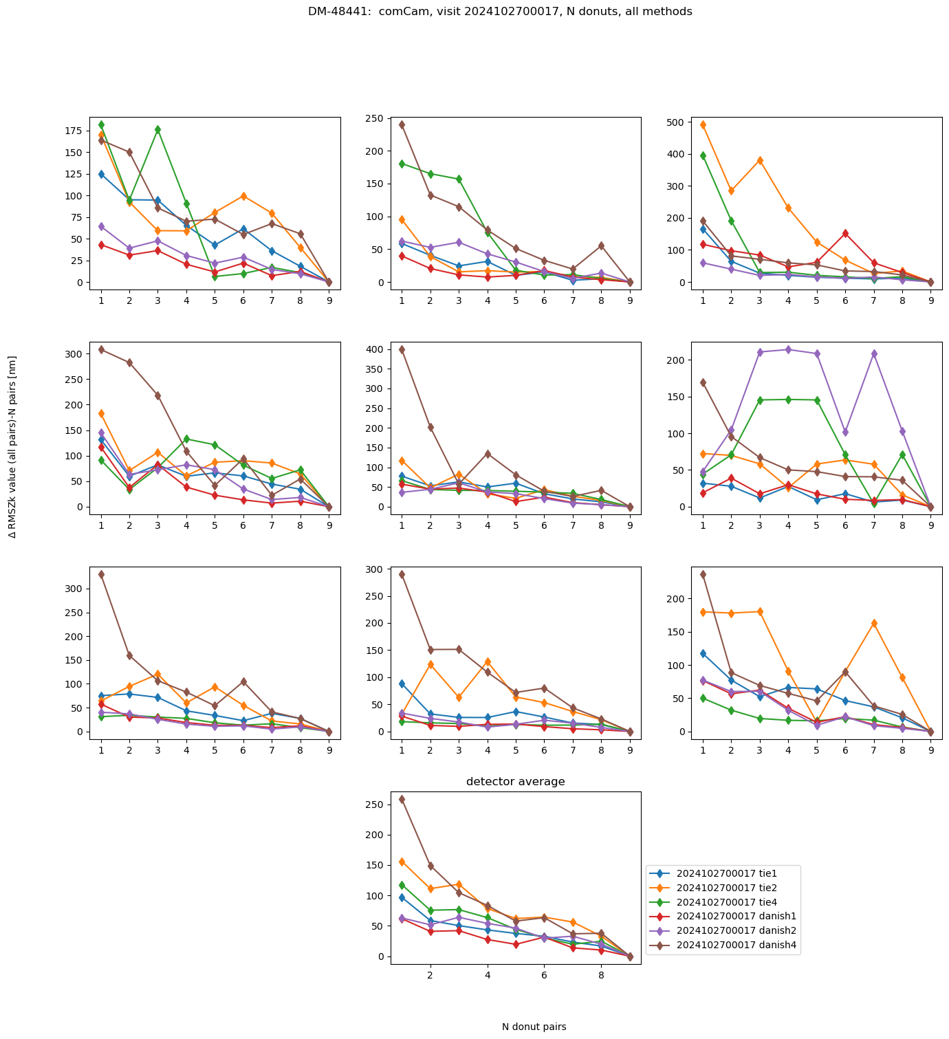
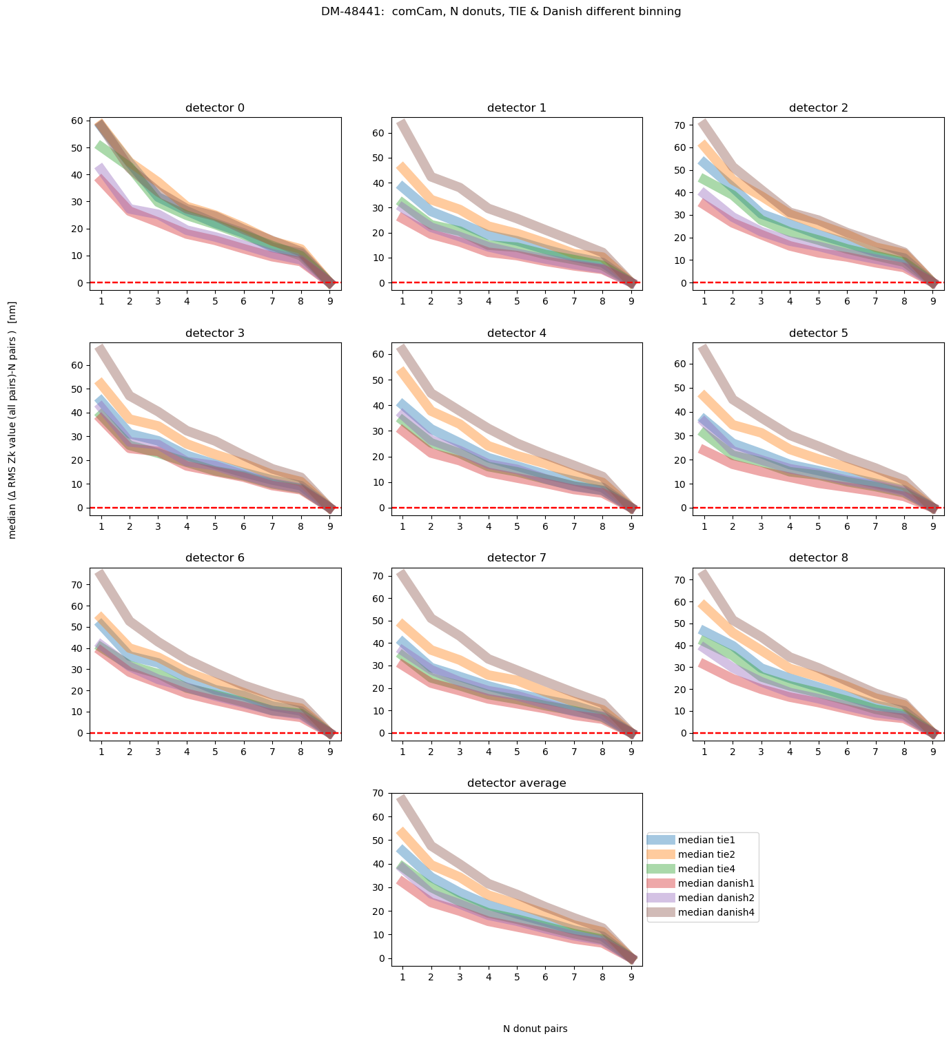
This rapidity of convergence can be summarized for each binning by taking an average across all visits:
file = f'u_scichris_aosBaseline_tie_danish_rms_visit_604.npy'
rms_visit = np.load(file, allow_pickle=True).item()
file = f'u_scichris_aosBaseline_tie_danish_rms_visit_asec_604.npy'
rms_visit_asec = np.load(file, allow_pickle=True).item()

all_visits_rms_per_method = {}
for method in results_visit[visit].keys():
    all_visits_rms_per_det = {}
    for i in range(9):
        all_visits_rms_per_det[i] = []
        for visit in rms_visit.keys():

          # plot the RMS diff for each detector
          rms_per_det =  rms_visit[visit][method][i]

          if len(rms_per_det) == 9:
            all_visits_rms_per_det[i].append(rms_per_det)
    all_visits_rms_per_method[method] = all_visits_rms_per_det

all_visits_rms_per_method_asec = {}
for method in results_visit[visit].keys():
    all_visits_rms_per_det_asec = {}
    for i in range(9):
        all_visits_rms_per_det_asec[i] = []
        for visit in rms_visit_asec.keys():

          # plot the RMS diff for each detector
          rms_per_det =  rms_visit_asec[visit][method][i]

          if len(rms_per_det) == 9:
            all_visits_rms_per_det_asec[i].append(rms_per_det)
    all_visits_rms_per_method_asec[method] = all_visits_rms_per_det_asec
Nvisits = len(list(rms_visit.keys()))
fig,axs = plt.subplots(4,3,figsize=(16,16))
ax = np.ravel(axs)
for method in results_visit[visit].keys():
    y_data = []
    x_data = range(1,10)
    for i in range(9):
        per_det_med =  np.nanmedian(all_visits_rms_per_method[method][i], axis=0)
        ax[i].plot(x_data,per_det_med, lw = 10, alpha=0.4,
                  label=f'median {method}')
        ax[i].axhline(0,ls='--', c='red')
        ax[i].set_xticks(np.arange(1,10, step=1))
        ax[i].set_title(f'detector {i}')
        y_data.append(per_det_med)

    ax[10].plot(x_data, np.mean(y_data, axis=0), lw = 10, alpha=0.4,
                  label=f'median {method}')
    ax[10].set_xticks(np.arange(1,10, step=1))
ax[10].legend(bbox_to_anchor=[1.,0.8], title='')
ax[10].set_title('detector average')
ax[9].axis('off')
ax[11].axis('off')


fig.text(0.5,0.05, 'N donut pairs')
fig.text(0.05,0.5,  'median ('+ r'$\Delta$ RMS'+' Zk value (all pairs)-N pairs )  [nm]', rotation='vertical')
fig.subplots_adjust(hspace=0.3)
fig.suptitle(f'DM-48441:  comCam, N donuts, TIE & Danish different binning ')
Text(0.5, 0.98, 'DM-48441: comCam, N donuts, TIE & Danish different binning ')
Nvisits = len(list(rms_visit.keys()))
fig,axs = plt.subplots(4,3,figsize=(16,16))
ax = np.ravel(axs)
for method in results_visit[visit].keys():

    y_data = []
    x_data = range(1,10)
    for i in range(9):
        per_det_median = np.nanmedian(all_visits_rms_per_method_asec[method][i], axis=0)
        ax[i].plot(x_data, per_det_median, lw = 10, alpha=0.4,
                  label=f'median {method}')
        ax[i].set_xticks(np.arange(1,10, step=1))
        ax[i].set_ylim(-0.001, 0.035)
        ax[i].axhline(0,ls='--', c='red')

        ax[i].set_title(f'detector {i}')
        y_data.append(per_det_median)

    ax[10].plot(x_data, np.mean(y_data, axis=0), lw = 10, alpha=0.4,
                  label=f'median {method}')
    ax[10].set_xticks(np.arange(1,10, step=1))
ax[10].legend(bbox_to_anchor=[1.,0.8], title='')
ax[10].set_title('detector average')
ax[9].axis('off')
ax[11].axis('off')

fig.text(0.5,0.05, 'N donut pairs')
fig.text(0.05,0.5,  'median ('+ r'$\Delta$ RMS'+' Zk value (all pairs)-N pairs )  [asec]', rotation='vertical')
fig.subplots_adjust(hspace=0.3)
fig.suptitle(f'DM-48441:  comCam, N donuts, TIE & Danish different binning ')
Text(0.5, 0.98, 'DM-48441: comCam, N donuts, TIE & Danish different binning ')
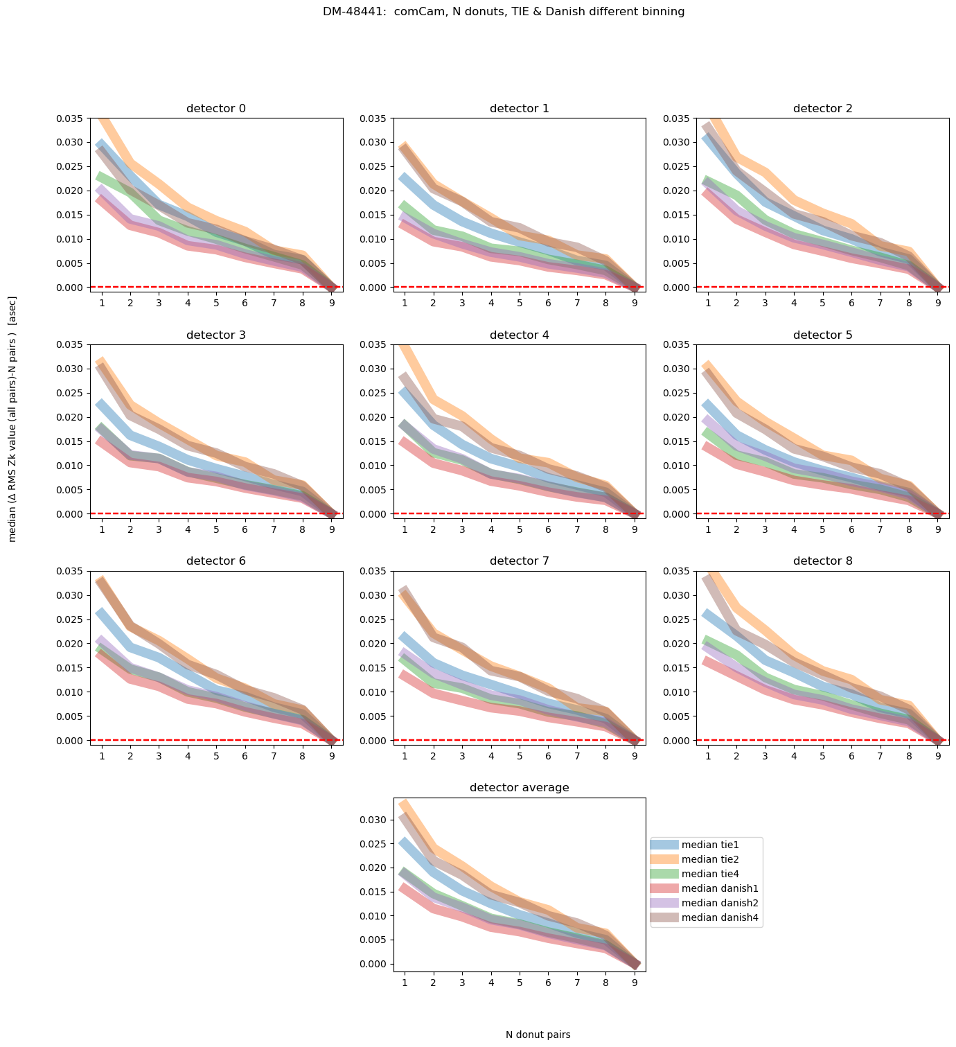
This shows us that, on average, Danish even with 2x binning achieves the final answer with less initial deviation than TIE. We can also plot different magnitude ranges:
file = f'u_scichris_aosBaseline_tie_danish_mag_visit_604.npy'
results_visit_mags = np.load(file , allow_pickle=True).item()
visits  = []
visit_mean_mag = []

Ndonuts = 9  # we take the mean only of the fisrt 9 donuts
for visit in results_visit_mags.keys():
    mean_per_det = []
    for detector in range(9):
        mags = results_visit_mags[visit][detector]['donutStampsExtraMag']
        if len(mags) < Ndonuts:

            mean_mag_per_det = np.mean(mags[:len(mags)])

        else:
            mean_mag_per_det = np.mean(mags[:Ndonuts])
        results_visit_mags[visit][detector][f'mean_{Ndonuts}_donuts']= mean_mag_per_det
        mean_per_det.append(mean_mag_per_det)
    visits.append(int(visit))
    visit_mean_mag.append(np.mean(mean_per_det))
fig = plt.figure(figsize=(7,5), dpi=150)

plt.hist(visit_mean_mag, histtype='step', bins=23)
plt.ylabel('Count')
plt.xlabel('Mean visit magnitude for N brightest donuts ')
plt.axvline(12, ls='--',c='red')
plt.axvline(13, ls='--',c='red')
<matplotlib.lines.Line2D at 0x7fbeffda5970>
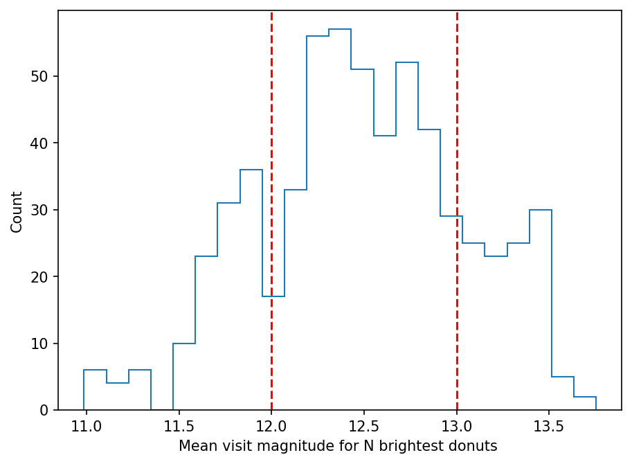
mag_ranges = [0,12,13,20]

mag_labels = [r'$\langle$'+'mag'+r'$\rangle$'+' < 12',
              '12 < '+r'$\langle$'+'mag'+r'$\rangle$'+' < 13',
              '13 < '+r'$\langle$'+'mag'
]

for idx in range(len(mag_ranges)-1):
    mag_min = mag_ranges[idx]
    mag_max = mag_ranges[idx+1]
    selected_visits = np.array(visits)[(mag_min < np.array(visit_mean_mag) ) * (np.array(visit_mean_mag) < mag_max)]
    all_visits_rms_per_method_asec = {}
    for method in results_visit[visit].keys():
        all_visits_rms_per_det_asec = {}
        for i in range(9):
            all_visits_rms_per_det_asec[i] = []
            for visit in selected_visits:

              # plot the RMS diff for each detector
              rms_per_det =  rms_visit_asec[visit][method][i]
              if len(rms_per_det) == 9:
                all_visits_rms_per_det_asec[i].append(rms_per_det)
        all_visits_rms_per_method_asec[method] = all_visits_rms_per_det_asec

    Nvisits = len(list(selected_visits))
    fig,axs = plt.subplots(3,3,figsize=(16,10))
    ax = np.ravel(axs)
    for method in results_visit[visit].keys():
        for i in range(9):
            ax[i].plot(range(1,10), np.nanmedian(all_visits_rms_per_method_asec[method][i], axis=0), lw = 10, alpha=0.4,
                      label=f'median {method}')
            ax[i].set_ylim(-0.001, 0.021)
            ax[i].axhline(0,ls='--', c='red')
            ax[i].set_xticks(np.arange(1,10, step=1))
        #ax[i].legend()
    ax[2].legend(bbox_to_anchor=[1.,0.6], title='')
    fig.text(0.5,0.05, 'N donut pairs')
    fig.text(0.05,0.5,  'median ('+ r'$\Delta$ RMS'+' Zk value (all pairs)-N pairs )  [asec]', rotation='vertical')
    fig.subplots_adjust(hspace=0.3)
    fig.suptitle(f'DM-48441:  comCam, {Nvisits} visits, '+mag_labels[idx]+ ', TIE & Danish different binning ')
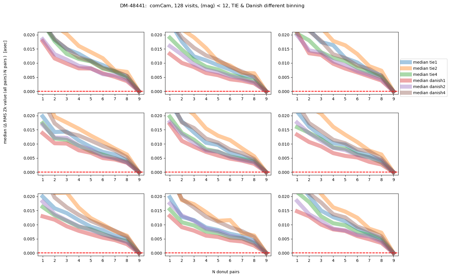
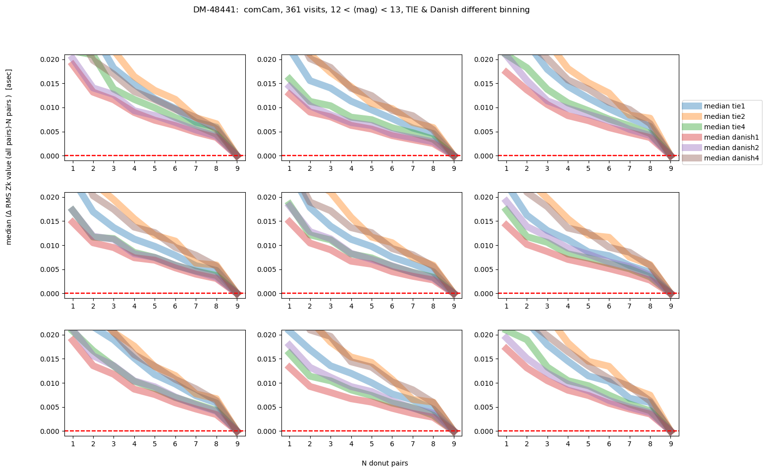
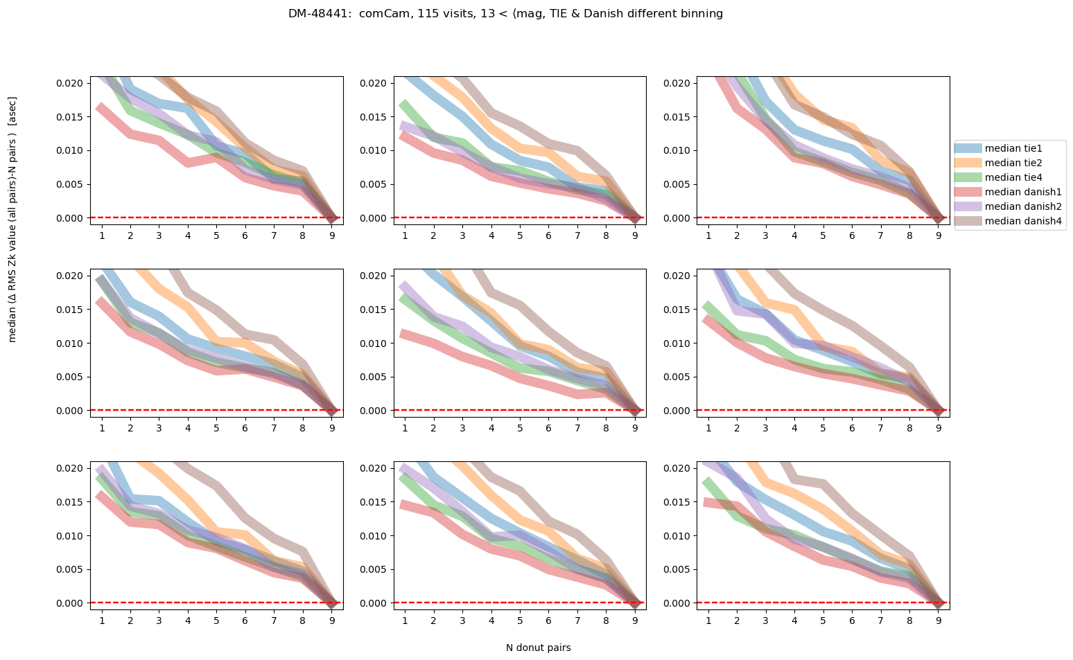
As we would expect, the brighter the donuts, the quicker the convergence to the final answer. Danish with (red and purple lines) outperforms TIE for edge detectors, but for center detector Danish with x2 binning achieves similar performance as TIE. Note however, that the “final answer” may be different for each binning, as each binning results in a slightly different wavefront estimation. In the next section we address what is the difference between the average of 9 donut pairs for each binning method.
Median of N donuts: same visit, different binning#
To compare Zernikes for the same visit but different binning levels, we average across 9 brightest donuts per detector:
fname = f'u_scichris_aosBaseline_tie_danish_zernikes_tables_604.npy'
results_visit = np.load(fname, allow_pickle=True).item()
# plotting
Nmin = 1
Nmax = 10
fig,axs = plt.subplots(3,3,figsize=(16,10))
ax = np.ravel(axs)

visit = list(results_visit.keys())[2]

for method in results_visit[visit].keys():
    results = results_visit[visit][method]
    # iterate over detectors
    for i in range(9):
        zernikes_all = results[i]
        # select only those zernikes that were actually used
        zernikes = zernikes_all[zernikes_all['used'] == True]

        # read the available names of Zk mode columns
        zk_cols = [col for col in zernikes.columns if col.startswith('Z')]
        zk_modes = [int(col[1:]) for col in zk_cols]

        # select not the stored average, which uses potentially all donuts
        # per detector, but instead calculate average using all available donuts
        all_rows = zernikes[Nmin:Nmax]
        zk_fit_nm_median = [np.median(all_rows[col].value) for col in zk_cols]

        ax[i].plot(zk_modes, np.array(zk_fit_nm_median), marker='d', label=f'{visit} {method}')
        ax[i].set_xticks(np.arange(4,29,step=2))


ax[2].legend(bbox_to_anchor=[1.,0.6], title='')
fig.text(0.5,0.05, 'Zk mode')
fig.text(0.05,0.5,  r'Mean Zk value [nm]', rotation='vertical')
fig.subplots_adjust(hspace=0.3)
fig.suptitle(f'DM-48441:  comCam, visit {visit}, N donuts, all methods ')
Text(0.5, 0.98, 'DM-48441: comCam, visit 2024102500123, N donuts, all methods ')
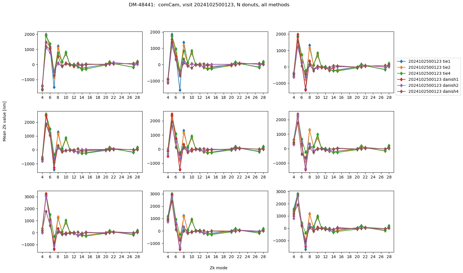
We find the RMS difference between average of 9 donut pairs with no binning, vs various binning settings.
def find_avg_zernikes_N_pairs(zernikes_all, Nmin=0, Nmax=10):

    # select only those zernikes that were actually used
    zernikes = zernikes_all[zernikes_all['used'] == True]

    # read the available names of Zk mode columns
    zk_cols = [col for col in zernikes.columns if col.startswith('Z')]

    # select not the stored average,
    # but calculate average using all available donuts

    all_rows = zernikes[Nmin:Nmax]
    zk_fit_nm_avg  = [np.median(all_rows[col].value) for col in zk_cols]

    return zk_fit_nm_avg
# calculation of RMS diff
Nmin=0

zk_diff_tie_danish = {}
for met in ['tie', 'danish']:
    zk_diff_all_visits = {}
    count =0
    for visit in tqdm(visits_available):
        zk_diff_per_visit = {}
        for method  in [f'{met}2', f'{met}4']:
            results_binned = results_visit[visit][method]
            results_base = results_visit[visit][f'{met}1']

            zk_diff_per_visit[method] = {}
            for i in range(9):
                # Find the mean for the baseline method
                zk_fit_nm_avg_base  = find_avg_zernikes_N_pairs(results_base[i])
                zk_fit_nm_avg_base_dense = makeDense(zk_fit_nm_avg_base, zk_modes)
                zk_fit_asec_base_dense = convertZernikesToPsfWidth(1e-3*zk_fit_nm_avg_base_dense)
                zk_fit_asec_base_sparse = makeSparse(zk_fit_asec_base_dense, zk_modes)

                # Find the mean for the binned method
                zk_fit_nm_avg_binned  = find_avg_zernikes_N_pairs(results_binned[i])
                zk_fit_nm_avg_binned_dense = makeDense(zk_fit_nm_avg_binned, zk_modes)
                zk_fit_asec_binned_dense =  convertZernikesToPsfWidth(1e-3*zk_fit_nm_avg_binned_dense)
                zk_fit_asec_binned_sparse = makeSparse(zk_fit_asec_binned_dense, zk_modes)

                # Calculate the RMS difference between the two
                rms_diff =  np.sqrt(
                                np.mean(
                                        np.square(
                                                    np.array(zk_fit_nm_avg_base) - np.array(zk_fit_nm_avg_binned)
                                                 )
                                       )
                               )
                # Calculate the same in ASEC
                rms_diff_asec =  np.sqrt(
                                np.mean(
                                        np.square(
                                                    np.array(zk_fit_asec_base_sparse) - np.array(zk_fit_asec_binned_sparse)
                                                 )
                                       )
                               )

                # Store both the per-mode differences and the RMS which is a single
                # number per visit - detector
                zk_diff_per_visit[method][i] = {'zk_no_binning_avg': zk_fit_nm_avg_base,
                                               'zk_with_binning_avg':zk_fit_nm_avg_binned,
                                                'zk_no_binning_avg_asec':zk_fit_asec_base_sparse,
                                                'zk_with_binning_avg_asec':zk_fit_asec_binned_sparse,
                                               'rms_diff':rms_diff,
                                                'rms_diff_asec':rms_diff_asec
                                               }
        # store the results for both methods per visit
        zk_diff_all_visits[visit] = zk_diff_per_visit
        count +=1
    zk_diff_tie_danish[met] = zk_diff_all_visits
100%|██████████| 572/572 [00:35<00:00, 15.97it/s]
100%|██████████| 572/572 [00:35<00:00, 16.00it/s]
We plot the difference between baseline for single visit:
# plotting
Nmin = 1

fig,axs = plt.subplots(3,3,figsize=(16,10))
ax = np.ravel(axs)


for method in [  'danish2', 'danish4',]:
    results = zk_diff_all_visits[visit][method]

    # iterate over detectors
    for i in range(9):
        # plot the RMS diff for each detector
        zernikes_avg_no_bin = results[i]['zk_no_binning_avg']
        zernikes_avg_bin = results[i]['zk_with_binning_avg']

        ax[i].plot(zk_modes, np.array(zernikes_avg_bin), marker='d', label=f'{visit} {method}')
        ax[i].plot(zk_modes, np.array(zernikes_avg_no_bin), marker='d', label=f'{visit} baseline')
        ax[i].set_xticks(np.arange(4,29,step=2))


ax[2].legend(bbox_to_anchor=[1.,0.6], title='')
fig.text(0.5,0.05, 'Zk mode')
fig.text(0.05,0.5,  r'Mean Zk value [nm]', rotation='vertical')
fig.subplots_adjust(hspace=0.3)
fig.suptitle(f'DM-48441:  comCam, visit {visit}, N donuts, danish binning x1, x2, x4 ')
Text(0.5, 0.98, 'DM-48441: comCam, visit 2024121100565, N donuts, danish binning x1, x2, x4 ')
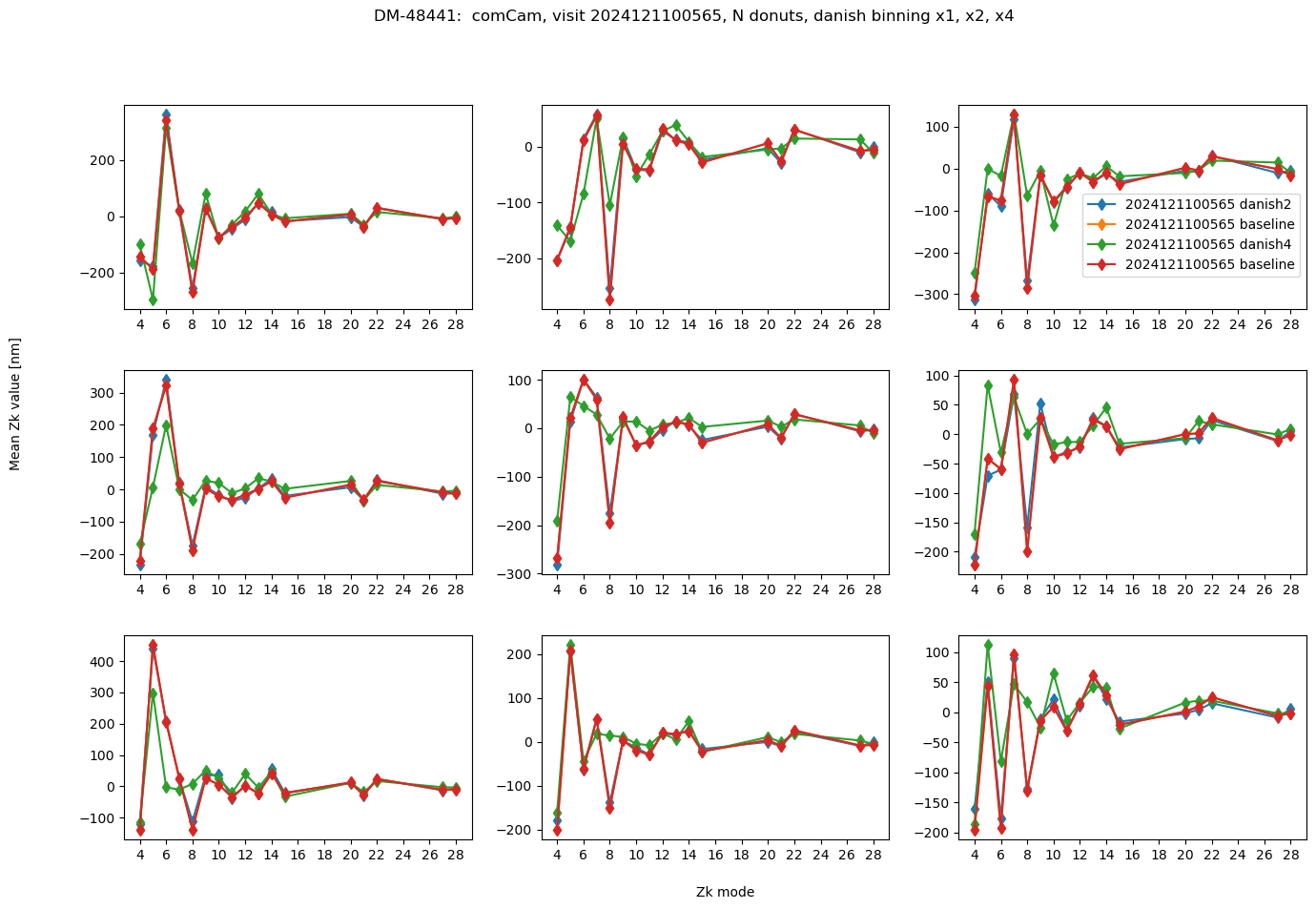
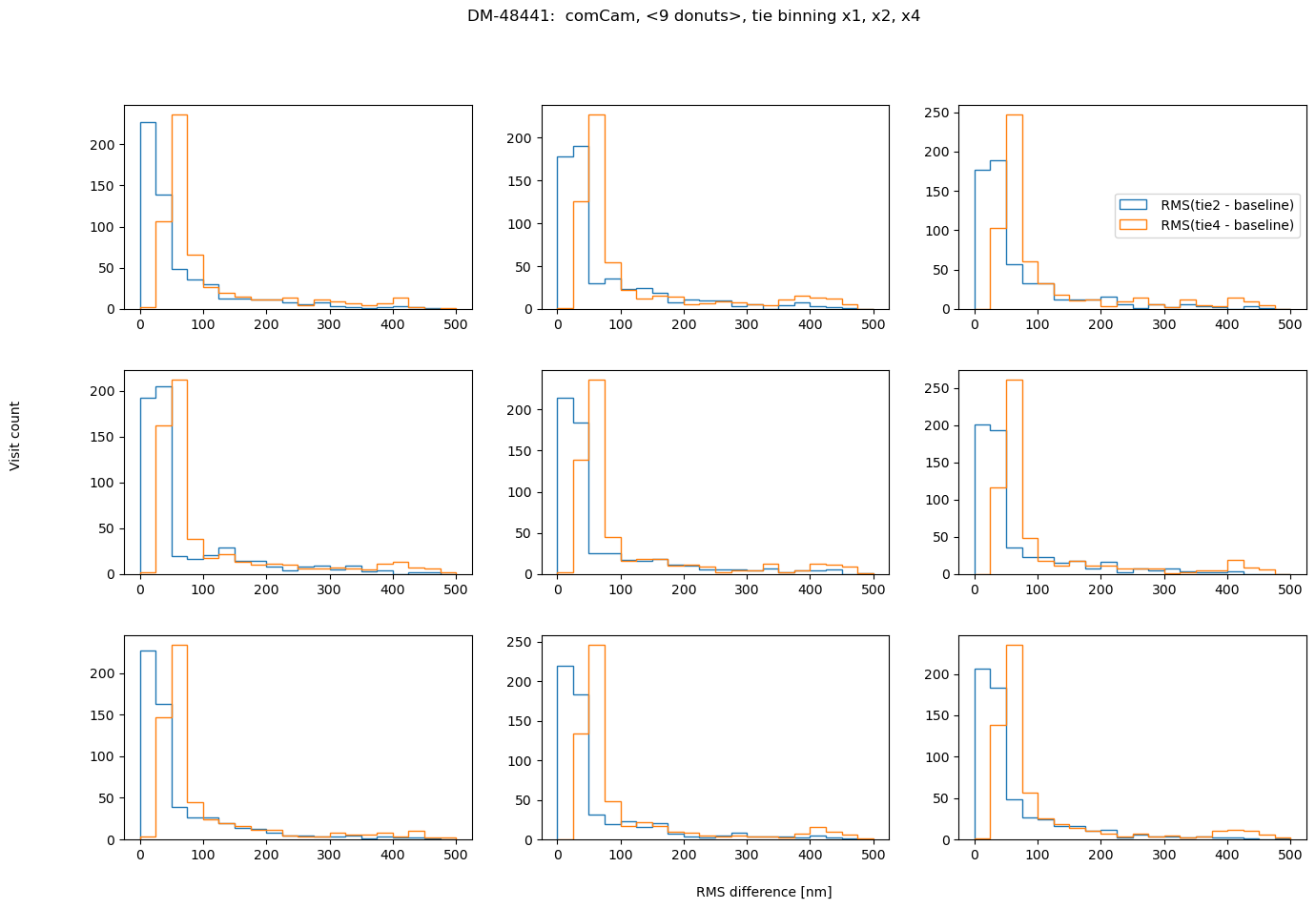
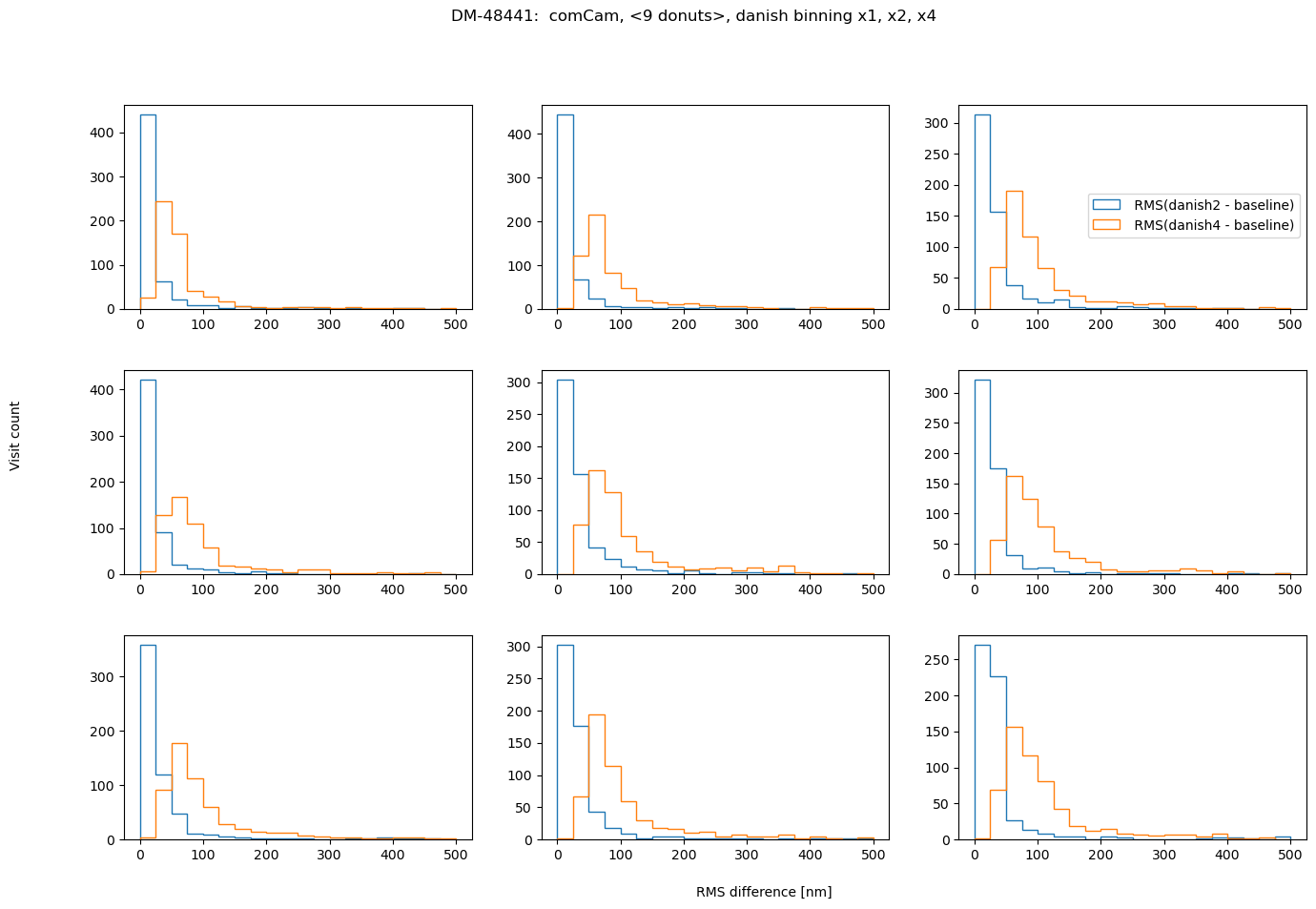
The results are really close (tens of nm). We now calculate the RMS difference between average of N donuts with different binning settings per detector-visit. We summarize that as a histogram for all visits:
rms_per_met = {}
for met in ['tie', 'danish']:

    rms_per_det = {}

    for i in range(9):
        rms_per_det[i] = {f'{met}2':[], f'{met}4':[]}


    for visit in zk_diff_tie_danish[met].keys():
        for method in [  f'{met}2', f'{met}4']:
            for i in range(9):
                results = zk_diff_tie_danish[met][visit][method][i]['rms_diff']
                rms_per_det[i][method].append(results)
    rms_per_met[met] = rms_per_det


Nvisits = len(zk_diff_tie_danish[met].keys())

# plotting
Nmin = 1
for met in ['tie', 'danish']:
    fig,axs = plt.subplots(3,3,figsize=(16,10))
    ax = np.ravel(axs)

    for i in range(9):
        for method in [  f'{met}2', f'{met}4']:
            ax[i].hist( rms_per_met[met][i][method], histtype='step', lw=3, bins=20, label=f' RMS({method} - baseline)',
                      range=[0,500])

    ax[2].legend(bbox_to_anchor=[1.,0.6], title='')
    fig.text(0.5,0.05, 'RMS difference [nm]')
    fig.text(0.05,0.5,  r'Visit count ', rotation='vertical')
    fig.subplots_adjust(hspace=0.3)
    fig.suptitle(f'DM-48441:  comCam, <9 donuts>, {met} binning x1, x2, x4 ')
also in asec:
rms_per_met = {}
for met in ['tie', 'danish']:

    rms_per_det = {}

    for i in range(9):
        rms_per_det[i] = {f'{met}2':[], f'{met}4':[]}


    for visit in zk_diff_tie_danish[met].keys():
        for method in [  f'{met}2', f'{met}4']:
            for i in range(9):
                results = zk_diff_tie_danish[met][visit][method][i]['rms_diff_asec']
                rms_per_det[i][method].append(results)
    rms_per_met[met] = rms_per_det


Nvisits = len(zk_diff_tie_danish[met].keys())

# plotting
Nmin = 1
for met in ['tie', 'danish']:
    fig,axs = plt.subplots(3,3,figsize=(16,10))
    ax = np.ravel(axs)

    for i in range(9):
        for method in [  f'{met}2', f'{met}4']:
            ax[i].hist( rms_per_met[met][i][method], histtype='step', lw=3, bins=20, label=f' RMS({method} - baseline)',
                      range=[0,0.4])

    ax[2].legend(bbox_to_anchor=[1.,0.6], title='')
    fig.text(0.5,0.05, 'RMS difference [asec]')
    fig.text(0.05,0.5,  r'Visit count ', rotation='vertical')
    fig.subplots_adjust(hspace=0.3)
    fig.suptitle(f'DM-48441:  comCam,  <9 donuts>, {met} binning x1, x2, x4 ')
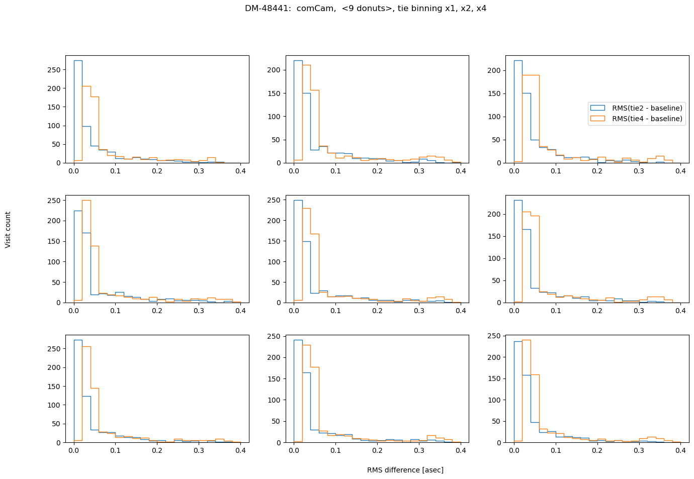
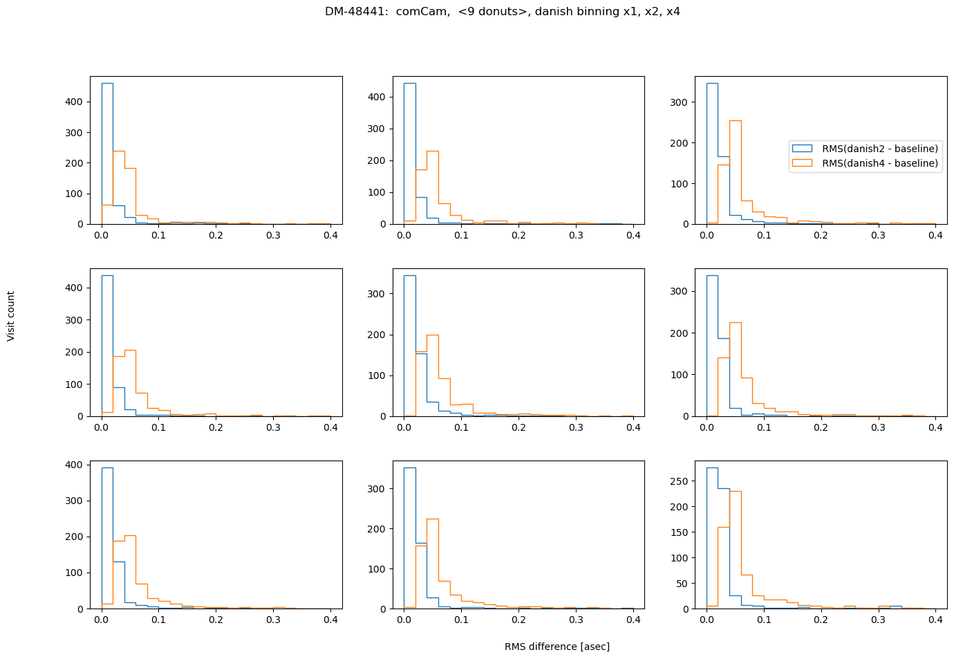
Summary#
In conclusion, choosing binning of x2 for either TIE or Danish vs no binning does not result in a significant RMS deviation (<0.1 asec). However, using binning x4 is not recommended for Danish as it causes twice as large RMS departure. Comparing the amount of information in 1 donut pair, increasing that all the way to 9 donut pairs, we note that for brighter mean magnitude (<12 mag), the median RMS departure is < 0.01 asec from the single donut pair to a median of 9 donut pairs. For all magnitude ranges, Danish more quickly arrives at the final answer (less donuts pairs necessary to achieve the same stability of estimated wavefront).